Worldwide Assessment of Energy Performance of PV-Integrated Rotating Residential Buildings

1. Introduction

Buildings account for 30–40% of global final energy consumption and a similar share of greenhouse gas emissions, making energy efficiency of the built environment a central component of climate-mitigation strategies [1, 2]. A substantial portion of the energy use of the building sector is driven by heating, cooling, and lighting end uses. While conventional design practices optimize building orientation based on prevalent climatic conditions, static building envelopes cannot adapt to daily or seasonal variations in solar radiation, limiting performance throughout the year, particularly in regions with pronounced seasonal changes [2, 3].

Recent advances in adaptive architecture have shown that dynamic elements such as movable shading devices and kinetic façades can improve thermal comfort and energy performance of buildings [4]. Extending the dynamic concept to whole-building rotation is technically feasible, as demonstrated by several real-world examples outlined in Table 1, including the Girasole House in Australia [5], the DrehHaus in Germany [6], and the English Wheelbarrow House in the Netherlands [7]. These structures mainly prioritize panoramic views rather than energy optimization, yet they demonstrate that azimuthal rotation is mechanically feasible and could potentially be leveraged to improve building energy performance.

While several rotating buildings have been constructed worldwide, most of them were primarily designed to enhance panoramic views or architectural novelty rather than to optimize building energy performance. Rotating restaurants and observation structures, for instance, commonly employ continuous rotation to provide 360° views of the surrounding environment, with little consideration given to energy efficiency. Only a limited number of residential rotating buildings exist, and their design motivations have generally focused on improving views or architectural flexibility rather than systematically reducing operational energy demand. Consequently, the potential of controlled building rotation as an adaptive strategy for reducing residential energy consumption remains largely unexplored in the existing literature.

A recent study by Krarti (2025) analyzed the energy demand of rotating US residential buildings integrated with rooftop PV systems, reporting a 21.7% reduction in HVAC energy end use in Phoenix, AZ, and showing that elongated geometries with high WWR benefit most from dynamic orientation [8]. The study also demonstrated that independent rotation of buildings and PV arrays can significantly decrease net energy needs. Indeed, PV tracking systems using single-axis and dual-axis rotations can achieve 20–60% higher energy production than fixed installations [9, 10, 11]. However, the adoption of PV tracking systems for residential settings remains limited, and their integration with rotating buildings has rarely been assessed. Despite these promising developments, existing literature on dynamic buildings and PV tracking systems still suffers from two main gaps:

(i) building rotation and PV tracking are often analyzed independently, preventing a full understanding of net annual performance of PV-integrated rotating buildings; and

(ii) most studies focus on a specific set of climates or design parameters, limiting their general applicability.

To address these gaps [8], the study presented in this paper introduces a unified simulation framework to evaluate the energy performance of PV-integrated rotating residential buildings across diverse design configurations and climate types. The analysis quantifies how building rotation influences heating and cooling demands, assesses the energy performance of rooftop PV systems under both fixed and tracking configurations, and examines the resulting net-energy balance for PV-integrated rotating buildings using various control strategies.

Table 1. Characteristics of reported existing rotating buildings

Building / Project	Location	Primary Purpose	Rotation Characteristics	Reported Energy-Related Performance	Ref.
Girasole House	Canberra, Australia	Residential	Solar-responsive azimuth rotation; low-power motor	Rotation consumes energy comparable to a small light bulb; improved passive heating/cooling	[5]
DrehHaus	Germany	Residential	Automated rotation based on solar path	Generates \(\sim\)10,000 kWh/year; consumes \(\sim\)7,000 kWh/year; \(\sim\)3,000 kWh surplus used for EV charging	[6]
English Wheelbarrow House	Netherlands	Residential	Planetary-inspired rotation; full 360° in \(\sim\)26 min	Improved natural lighting and passive heat gains; qualitative energy improvements	[7]
Revolving Restaurants	Worldwide	Commercial	Continuous rotation for panoramic views	Not designed for energy optimization; no reported energy performance data	[12]

2. Analysis Framework

This section describes the modeling framework used to evaluate the energy performance of rotating residential buildings with and without rooftop photovoltaic (PV) systems. The objective of the modeling framework is to quantify the impacts of various dynamic orientation strategies on space heating and cooling demands and PV generation yields, as well as the effects of different building geometries and envelope characteristics.

The main components of the simulation environment are described in the following sections, including the analysis tools, building energy models, and control strategies. Because EnergyPlus cannot simulate physical rotation directly, each building is modelled at 16 discrete orientations (22.5° increments). Dynamic rotation strategies, monthly, daily, and hourly, are evaluated and optimized using the Distinct Building Energy Modeling (DBEM) approach outlined by Krarti [8].

The DBEM approach consists of performing a series of quasi-steady building energy simulations for a set of discrete building orientations that collectively represent the full 360° rotation. The thermal performance of the rotating building is then estimated by combining the simulation results obtained for each stationary orientation according to the selected rotation control strategy (i.e., monthly, daily, or hourly rotation). This approach provides a practical method for approximating the energy performance of kinematically dynamic buildings using conventional whole-building simulation tools such as EnergyPlus.

The modeling approach in this study involves several simplifying assumptions that should be acknowledged. First, building rotation is simulated using 16 discrete orientation angles (22.5° increments), consistent with the DBEM approach described above and adopted in previous studies [8]. This discretization is required due to the limitations of EnergyPlus, which does not support continuous rotation. While this method enables the evaluation of dynamic orientation strategies, it represents an approximation of a continuous rotation process and may introduce minor deviations in the predicted energy performance. Nevertheless, the selected angular resolution provides a reasonable balance between computational efficiency and accuracy for comparative analysis.

In addition, photovoltaic (PV) electricity generation is estimated using PVWatts, a widely used tool for preliminary PV performance assessment. Although PVWatts provides reliable estimates of annual and hourly PV output, it does not account for certain factors such as detailed shading effects, dynamic system losses, or advanced control strategies. Therefore, the PV performance results presented in this study should be interpreted as representative estimates rather than exact predictions.

Overall, the adopted modeling framework is intended to support comparative analysis across different rotation and PV configurations and to identify general performance trends, rather than to provide highly detailed predictions for specific dynamic building designs.

2.1 Building Model Description

The residential building models considered in this study are adapted from standard Belgian single-family homes [13]. Table 2 summarizes main model features, including internal loads, HVAC settings, and window-to-wall ratios (WWR), while Table 3 lists the construction assemblies and thermophysical properties of the building envelopes.

Table 2. Main features of the residential building energy model

Building Model Parameters Used for Energy Analysis
Floor surface Area [\(m^2\)]	100- 252
Wall height [m]	3
Window	Double
Window to wall ratio [%]	31% – 80%
Heating operation	October – May HSPF: 11.9 Setpoint: 20°C
Cooling operation	June – September COP: 3.5 Setpoint 26°C
Ventilation rate [\(m^3\)/h]	0.15
ACH [%]	100%
Infiltration rate [\(m^3\)/h.\(m^2\)] at 50 Pa	2
People density [ppl]	2
Lighting density [W/\(m^2\)]	2.86
Equipment density [W/\(m^2\)]	4.7
Cooking range [W]	5000
DHW range [W]	625

Table 3. Construction assemblies and thermophysical properties of building envelope components.

Material	Thickness [mm]	Conductivity [W/m.K]	Density [kg/\(m^3\)]	Specific Heat [J/kg.K]
Roof
Pantile	10	0.71	1800	1000
Fiber-cement panel	3	0.25	1200	1470
Mineral wool insulation	300	0.045	175	1030
Membrane	5	0.23	1100	1000
Air layer	20	0.316	1.204	1006
Plaster	10	0.52	1300	1000
Exterior walls
Brick	90	0.71	1800	1000
Air layer	30	0.025	1.204	1006
Mineral wool insulation	150	0.045	175	1030
Sand-lime brick	140	0.45	1200	1000
Plaster	20	0.52	1300	1000
Floor
Lightweight concrete	100	0.55	1200	1000
Reinforced concrete	200	1.7	2400	1000
PUR insulation	100	0.035	30	1400
Screed	50	0.55	1200	1000
Ceramic tile	15	0.81	2000	1000

To better reflect the airtightness standards of high-performance Belgian housing, an infiltration rate of 2 m³/h·\(m^2\) at 50 Pa is adopted in this study. This value is supported by Vandenbogaerde et al. [14], who evaluated airtightness across 30 dwellings in Flanders, and provides a more representative benchmark than the conservative default values typically used in other studies.

The building energy models used in this study are based on standard residential building characteristics and validated assumptions reported in the literature [13, 14]. The objective of the analysis is to perform a comparative evaluation of different rotation strategies and PV integration configurations using representative building layouts rather than to predict the exact energy demands for specific buildings.

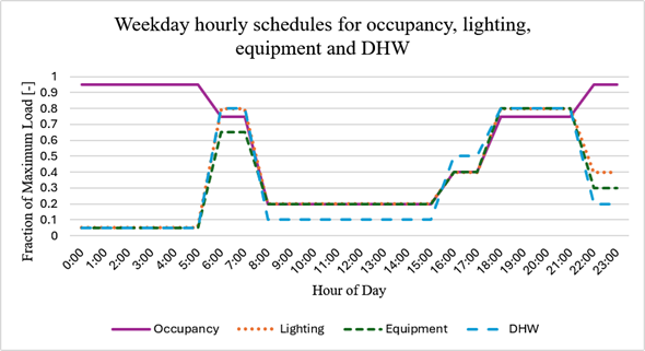
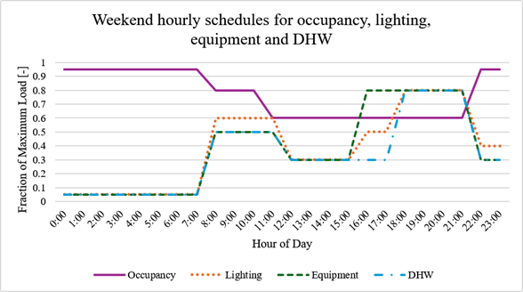
Moreover, time-dependent hourly schedules are applied to occupancy, lighting, and equipment to reflect typical residential usage patterns. In addition, indoor temperature setback schedules are implemented to reflect daily and weekly occupancy patterns.

The hourly schedules used for occupancy, lighting, equipment, and domestic hot water (DHW) are illustrated in Figure 1 and Figure 2 for typical weekend and weekend conditions. These schedules reflect typical residential usage patterns, with lower activity during working hours on weekdays and more evenly distributed occupancy and equipment use during weekends.

2.2 Building Geometries Configurations and Rotation Methodology

To evaluate the impact of geometry, scale, and dynamic orientation on thermal performance, five residential building models are considered as part of a preliminary sensitivity analysis. All building configurations have the same construction assemblies, material properties, and internal loads described in Section 2.1, ensuring a consistent basis for comparative analysis. Variations between building models include floor area, shape, and window-to-wall ratio (WWR), as detailed in Table 4.

All housing unit models have windows located on a single façade, consistent with previous studies on rotating buildings [8], which adopt similar configurations to isolate the impact of building orientation on energy performance. This simplified and directional configuration allows for a clearer evaluation of the effects of dynamic rotation strategies. In typical residential buildings, where windows are distributed across multiple façades, the impact of orientation on annual energy demand is reduced, and thus any associated benefits of kinematically dynamic buildings are therefore expected to be lower. To evaluate the thermal impacts of building rotation, 16 orientation settings, spaced at 22.5° intervals, are considered. The orientation settings are adjusted using three setting frequencies: monthly, daily, or hourly. The adjustments are based on minimizing the annual energy demand for the rotating housing unit.

Table 4. Geometric configurations considered for residential building models

ID		Shape	Area [\(m^2\)]	WWR	S/V Ratio	Static Orientation [°]
S1		Square 15 m x 15 m	225	0.31	0.93	180
S2		Square 15 m x 15 m	225	0.8	0.93	180
S3		Square 10 m x 10 m	100	0.8	1.07	180
O1		Octagone 8 boders of 6 m	252	0.8	0.9	180
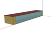
R1		Rectangle 20 m x 5 m	100	0.8	1.17	180

This framework enables consistent evaluation of rotation strategies across shapes, climates, and envelope characteristics, forming the basis for the following analysis.

2.3 PV System Modeling and Tracking Configurations

Rooftop PV performance is evaluated for different tracking strategies using PVWatts Calculator [15]. For this study, four rooftop PV system configurations are considered:

• Fixed systems: Panels are installed at a static tilt and azimuth, typically facing equatorward (e.g. South in the Northern Hemisphere) at a fixed optimal angle.
• Single-axis tilt tracking: Panels rotate along a horizontal axis (typically aligned North–South) to follow the sun’s daily motion from East to West.
• Single-axis azimuth tracking: Here, panels rotate horizontally to follow the sun’s azimuthal path, while maintaining a constant tilt.
• Dual-axis tracking: The most dynamic configuration, these systems adjust both tilt and azimuth in real-time, maintaining perpendicularity to the sun throughout the day and year.

2.4 Integrated PV-Building Performance Methodology

To evaluate how building rotation interacts with rooftop photovoltaic (PV) systems, three integrated scenarios are evaluated by combining the thermal building models described in Sections 2.1 and 2.2 with the PV configurations outlined in Section 2.3. PV-integrated rotating buildings are evaluated using the net annual electricity balance as the main performance metric. This balance is computed for multiple combinations of rotation control frequencies (monthly, daily, and hourly) and PV tracking configurations. The results are then used to quantify the relative benefits of coordinated control versus independent operation of building rotation and PV tracking.

All building thermal and energy simulations are performed using EnergyPlus through the OpenStudio interface [16]. For each building configuration, hourly heating, cooling, lighting equipment, and domestic hot water demands are first simulated for a set of discrete building orientations. The DBEM approach is then used to combine these simulation results according to the selected rotation strategy (monthly, daily, and hourly), allowing the estimation of total building electricity demand for dynamically oriented buildings.

Similarly, hourly PV generation is calculated using PVWatts for fixed, single-axis, and dual-axis tracking systems. For tracking systems, parasitic electricity consumption is modeled as a percentage of the PV electricity generation to account for motor operation and control systems. Based on reported values in the literature, tracking-related energy consumption typically ranges from approximately 3% to over 10% of gross PV electricity output, depending on system type and control strategy [9, 10, 11]. In this study, a constant parasitic loss of 6.5% of the PV electricity production is assumed for both single-axis and dual-axis tracking systems. This value represents a conservative estimate within the reported range and is consistent with intermittently actuated tracking systems [11], while remaining slightly higher than laboratory-based values reported in [9, 10].

Three integrated PV building configurations are evaluated in this study including:

• Scenario A: Fixed building + dual-axis PV tracking. The house remains static, while the PV system tracks both azimuth and tilt angles for optimal solar capture.
• Scenario B: Rotating building + roof-mounted PV. The building rotates using monthly, daily, and hourly adjustments, while the PV system remains fixed to the roof, providing passive azimuth tracking.
• Scenario C: Independently rotating building and PV system. The house rotates to minimize its annual heating and cooling energy demands, while the PV system operates independently with dual-axis tracking, offering maximum annual electricity yield.
• For Scenarios B and C, electricity required for rotating the building is accounted for as part of its total annual electricity demand, using the building energy modeling approach described in Section 2.5. Net energy demand for static or a rotating building is estimated as the difference between annual PV generation yield and total building electricity use. Moreover, hourly, daily, and monthly balances are further computed to identify seasonal mismatches as well as to optimize rotation adjustments.

This integrated framework provides a consistent basis for comparing the performance of rotating and non-rotating buildings under different PV strategies and climates, supporting evidence-driven decisions on PV sizing, rotation control frequency, and the practical considerations for designing and operating rotating residential buildings.

2.5 Electricity Demand for Building Rotation

To ensure realistic net energy assessments, the electricity required to rotate the building is accounted for when estimating the total energy consumption for Scenarios B and C (rotating configurations), in contrast with Scenario A (static). Rotation energy demands are determined based on data reported for a rotating home located in San Diego [17], featuring a 270,000 kg circular floor platform driven by a 1.5 hp motor. The system runs continuously at 0.75 hp and completes a 360° rotation in approximately 33 minutes, consuming 0.31 kWh of electricity per full turn. This case study provides specific energy performance data and design specifications for one of the few documented real-world rotating residential buildings. While this case study allows for an estimation of the order of magnitude of the electricity required for building rotation, the actual energy demand may vary depending on several factors such as the total building mass, structural system, bearing configuration, and rotation mechanism. Therefore, the adopted values should be interpreted as indicative estimates intended to evaluate the relative impact of rotation strategies rather than precise predictions for a specific building configuration.

The rotation energy consumption is assumed to be proportional to the angular displacement of the building, allowing the calculation of energy use for different orientation strategies (monthly, daily, or hourly) based on the cumulative rotation required over time. The total rotation energy demand is obtained by summing the energy associated with each orientation adjustment throughout the simulation period. As a result, more frequent rotation strategies lead to higher cumulative rotation energy demands.

3. Energy Performance of Rotating Buildings

In this section, the impacts of various design specifications and control settings on the energy performance of rotating buildings, without rooftop PV systems, are discussed. Specifically, the effects of geometry configurations and window sizes as well as on the frequency of rotation are evaluated for two representative climates, Boulder, CO, characterized by semi-arid climate with high solar radiation, and Brussels, Belgium, featuring a temperature climate with low solar radiation especially during the winter.

3.1 Impact of Building Orientation

This section evaluates the effect of orientation on thermal energy performance under both static and rotating conditions. The initial analysis is conducted for Boulder, CO, considering two building shapes:

• The square housing unit model (S2), 15 m × 15 m with WWR of 0.80, and
• The rectangular housing unit model (R1), 20 m × 5 m, also with WWR 0.80.

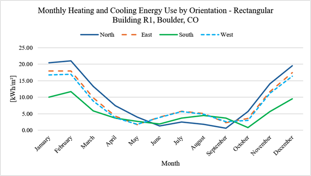
First, the annual energy demand for each building configuration is determined for 16 fixed orientations (i.e., 0° to 337.5° using 22.5° increments). Figure 3 and Figure 4 illustrate the annual heating/cooling energy end-use per unit floor area for static S2 and R1 housing unit models in Boulder, CO, for the four cardinal orientations.

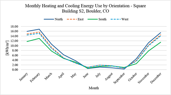
As shown in Figure 3, a south orientation reduces heating demand of the square housing unit (S2) during the winter months, reaching up to 26% in January compared to North-facing (i.e., from 15.92 kWh/m2 to 11.71 kWh/m2). However, during the summer months, cooling demand increases when facing south, reaching up to 91% in August, compared to north oriented housing unit due to higher solar heat gains.

Similar results are observed for a rectangular shape housing unit (R1) as illustrated in Figure 4. In fact, the rectangular unit R1 shows even greater sensitivity to orientation with a reduction of 51% in heating demand from 20.37 kWh/\(m^2\) for north-facing housing unit to 10.04 kWh/\(m^2\) for a south-facing unit. In addition, the cooling demand is increased by 148% in August when the housing unit is oriented south instead of north jumping from 1.8 kW/m2 to 4.47 kWh/\(m^2\).

These results indicate the important effects of orientation for the glazed façades on the heating and cooling demands for residential buildings.

To reduce seasonal mismatches, dynamic orientation strategies can be considered using various adjustment frequencies. The annual performance for a rotating housing unit model R1 is estimated using monthly, daily, and hourly adjustment settings. Figure 5 indicates the monthly optimal orientation settings to minimize the annual energy demand for the housing unit R1 in Boulder, CO.

As shown in Figure 5, the optimal monthly rotation settings call for the glazed façade to be south-facing (i.e., 180o) during winter months to maximize solar heat gains, and north-facing (i.e., 0o) during summer months minimizing solar heat gains. During the swing months, the optimal orientations range from south-east to south-west (i.e., 112.5° to 225°) to balance heating and cooling needs. The optimal monthly settings reduce the annual energy use of the housing unit model R1 by 14.2% compared to the static optimal orientation (i.e., south facing) when located in Boulder, CO.

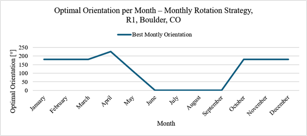
Figure 6 summarizes the annual distribution of optimal orientation settings for rotating housing unit model R1 in Boulder, CO, when adjusted monthly, daily, and hourly to minimize the annual energy demands.

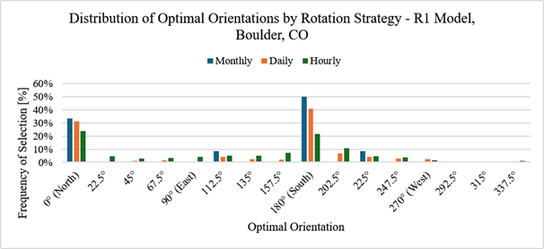
As shown in Figure 6, both north and south orientations for the glazed facades are the most dominant optimal settings for all the adjustment frequencies. North orientation is selected during the summer months, and south is used during the winter months. During the swing periods, other orientations are considered to minimize energy demands for heating and cooling. Typically, hourly orientation adjustment has a wide spread of settings following mostly the sun position throughout the year.

As expected, hourly rotation adjustment offers the highest annual energy savings for the housing unit model R1 reaching up to 17.8%, as indicated in Table 5 for buildings in Boulder, CO. Daily and monthly adjustments of the rotating housing units result in respectively 15.1% and 14.2% reductions of annual building energy demands compared to their static south-facing positions. For buildings in Belgium, the energy benefits of rotating buildings are lower with the highest reduction in annual energy consumption is estimated for hourly rotation adjustment frequency for R1 housing model as summarized in Table 6.

3.2 Impact of Building Shape

The shape of a building affects its solar exposure and therefore its heating and cooling needs. To evaluate the influence of shape on the annual energy performance of both static and rotating buildings, a set of geometries summarized in Table 7 are considered using the climatic conditions of Boulder, CO. The evaluated geometries include one- and two-story housing units of square, rectangular, and octagonal shapes with a fixed story height of 3 m having the same window-to-wall ratio (WWR).

The annual heating and cooling energy end-uses for each housing unit model is estimated for four cases: one optimal static orientation (i.e., south or 180°) and three rotating options using monthly, daily, and hourly orientation settings. Table 8 presents the annual heating and cooling energy demand results for all evaluated configurations.

The findings summarized in Table 8 confirm that dynamic rotation improves the annual energy performance of housing units for all shapes, with hourly rotation consistently yielding the highest annual energy demand reductions. However, the extent of the benefit varies significantly with geometry.

• Compact forms such as the square models (S1, S2) and octagon (O1) show limited sensitivity to rotation, with savings below 2% even for hourly orientation adjustments.
• Elongated or multi-story buildings, especially the two-story rectangles R2 and R3, achieve the highest energy benefits, with reductions up to 24% compared to their static orientation. These buildings with their extended façades offer more responsive surface area to solar shifts throughout the year.

These results highlight that rotation is most effective for shapes with strong directional dependence, such as narrow, elongated forms. In contrast, symmetrical or compact shapes benefit less due to their uniform orientation exposure.

Table 5. Annual space heating and cooling energy use for rotating housing units in Boulder, CO

ID		Orientation Strategy	Space Heating and Cooling Energy [kWh/\(m^2\)/year]	Reduction vs Fixed [%]
S1		Fixed Optimal	78.10	–
		Monthly Rotation	77.23	1.1%
		Daily Rotation	77.16	1.2%
		Hourly Rotation	76.89	1.5%
S2		Fixed Optimal	66.38	–
		Monthly Rotation	63.92	3.7%
		Daily Rotation	63.68	4.1%
		Hourly Rotation	62.80	5.4%
S3		Fixed Optimal	74.16	–
		Monthly Rotation	70.11	5.5%
		Daily Rotation	69.75	5.9%
		Hourly Rotation	68.43	7.7%
O1		Fixed Optimal	61.16	–
		Monthly Rotation	58.57	4.2%
		Daily Rotation	58.34	4.6%
		Hourly Rotation	57.26	6.4%
R1		Fixed Optimal	63.88	–
		Monthly Rotation	54.80	14.2%
		Daily Rotation	54.24	15.1%
		Hourly Rotation	52.52	17.8%

3.3 Impact of Window-to-Wall Ratio (WWR)

The effects of window size or window-to-wall ratio (WWR) on the energy performance of static and rotating buildings are assessed using the housing unit R1 model (20 m × 5 m) in Boulder, CO. For this building model, the window size is adjusted so its WWR varies from 0.1 to 0.9. Moreover, the orientation settings are optimized for static building models as well as monthly, daily, and hourly rotating building models. In the analysis, all other design and operating parameters are held constant.

Table 9 presents the annual heating and cooling demands for the evaluated cases. As expected, the analysis results show that increasing WWR reduces winter heating needs due to higher solar gains but increases summer cooling loads. However, the winter energy savings outweigh summer energy penalties, leading to a net decrease in annual building energy demand due to the dominantly cold climate of Boulder, CO.

The impact on energy performance of rotating buildings increases with higher WWR. With low WWR values (i.e., from 0.1 to 0.3), hourly rotation of the housing unit R1 reduces its annual energy use by less than 5%. In contrast, for high WWR (i.e., 0.8 and 0.9), hourly rotation of the housing unit R1 yields reductions of up to 20.5% in its annual energy needs. These results confirm that buildings with large, glazed façades benefit significantly from rotational strategies that align with seasonal variations in solar heat gains [8].

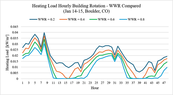
Figure 7 illustrates the hourly variations of heating demand during winter days (Jan 14–15) for various WWR values. The results of Figure 7 indicate that the heating needs consistently decrease with increasing WWR, with significantly lower demands observed for WWR values of 0.6 and 0.8 compared to the case of WWR=0.2. These results reflect the enhanced impact of the solar gains associated with larger glazed facades.

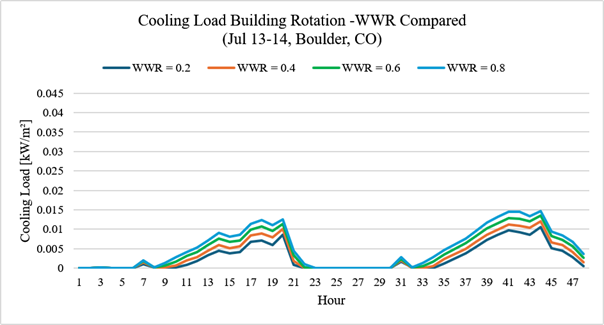
Similarly, Figure 8 highlights the hourly variations of the cooling loads for rotating housing units (R1 model) for various WWR values during the summer period (i.e., July 13–14) in Boulder, CO. Figure 8 shows that cooling loads increase with WWR for all the cases. Higher peaks are observed for WWR of 0.6 and 0.8, especially during afternoon hours. While rotation helps the housing units to reduce their solar heat gains during the summer, it cannot fully offset their impact in increasing cooling loads especially for larger glazed facades.

Table 6. Annual space heating and cooling energy use for rotating housing units in Brussels, Belgium

ID		Orientation Strategy	Space Heating and Cooling Energy [kWh/\(m^2\)/year]	Reduction vs Fixed [%]
S1		Fixed Optimal	73.58	–
		Monthly Rotation	73.46	0.2%
		Daily Rotation	73.11	0.6%
		Hourly Rotation	72.84	1.0%
S2		Fixed Optimal	69.21	–
		Monthly Rotation	68.54	1.0%
		Daily Rotation	68.21	1.4%
		Hourly Rotation	67.85	2.0%
S3		Fixed Optimal	76.48	–
		Monthly Rotation	75.06	1.9%
		Daily Rotation	74.35	2.8%
		Hourly Rotation	73.45	4.0%
O1		Fixed Optimal	62.09	–
		Monthly Rotation	61.34	1.2%
		Daily Rotation	61.16	1.5%
		Hourly Rotation	60.87	2.0%
R1		Fixed Optimal	75.58	–
		Monthly Rotation	72.00	4.7%
		Daily Rotation	71.60	5.3%
		Hourly Rotation	70.98	6.1%

Table 7. List of static and rotating building geometries considered for Boulder, CO

ID		Shape	Area [\(m^2\)]	WWR	S/V Ratio	Best Orientation [°]
S1		Square 15 m x 15 m	225	0.31	0.93	180
S2		Square 15 m x 15 m	225	0.8	0.93	180
S3		Square 10 m x 10 m	100	0.8	1.07	180
S4		2-Stories Square 10 m x 10 m	200	0.8	0.73	180
O1		Octagon with 8 Sides of 6 m	252	0.8	0.9	180
O2		Octagon with 8 Sides of 4 m	224	0.8	0.51	180
R1		Rectangle 20 m x 5 m	100	0.8	1.17	180
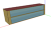
R2		2-Stories Rectangle 20 m x 5 m	200	0.8	0.83	180
R3		2-Stories Rectangle 10 m x 5 m	100	0.8	0.93	180

3.4 Impact of Glazing Type

This section examines the effects of glazing properties on the energy performance of rotating residential buildings. Three glazing types are considered for the housing unit R1 model in Boulder, CO, using four configurations including static orientation and monthly, daily, and hourly rotation adjustments. The three glazing types include:

• Single glazing: 3 mm clear float glass with poor insulation (U \(\approx\) 5.6 W/\(m^2\)·K, SHGC \(\approx\) 0.85)
• Double glazing: Two 3 mm panes with a 12 mm argon-filled cavity (U \(\approx\) 1.1 W/\(m^2\)·K, SHGC \(\approx\) 0.65)
• Low-E double glazing: Same configuration as double glazing but with a soft Low-E coating (U \(\approx\) 1.1 W/\(m^2\)·K, SHGC \(\approx\) 0.55)

All glazing values reflect typical residential performance using IGDB and ISO standards [18, 19].

Table 8. Annual space heating and cooling demand for each building shape under different rotation strategies in Boulder, CO

ID		Orientation Strategy	Space Heating and Cooling Energy [kWh/\(m^2\)/year]	Reduction vs Fixed [%]
S1		Fixed Optimal	78.10	–
		Monthly Rotation	77.23	-1.1%
		Daily Rotation	77.16	-1.2%
		Hourly Rotation	76.89	-1.5%
S2		Fixed Optimal	66.38	–
		Monthly Rotation	63.92	-3.7%
		Daily Rotation	63.68	-4.1%
		Hourly Rotation	62.80	-5.4%
S3		Fixed Optimal	74.16	–
		Monthly Rotation	70.11	-5.5%
		Daily Rotation	69.75	-5.9%
		Hourly Rotation	68.43	-7.7%
S4		Fixed Optimal	53.52	–
		Monthly Rotation	49.10	-8.3%
		Daily Rotation	48.81	-8.8%
		Hourly Rotation	45.04	-15.8%
O1		Fixed Optimal	61.16	–
		Monthly Rotation	58.57	-4.2%
		Daily Rotation	58.34	-4.6%
		Hourly Rotation	57.26	-6.4%
O2		Fixed Optimal	49.95	–
		Monthly Rotation	45.34	-9.2%
		Daily Rotation	45.10	-9.7%
		Hourly Rotation	43.81	-12.3%
R1		Fixed Optimal	63.88	–
		Monthly Rotation	54.80	-14.2%
		Daily Rotation	54.24	-15.1%
		Hourly Rotation	52.52	-17.8%
R2		Fixed Optimal	44.17	–
		Monthly Rotation	34.80	-21.2%
		Daily Rotation	34.52	-21.8%
		Hourly Rotation	33.59	-24.0%
R3		Fixed Optimal	53.70	–
		Monthly Rotation	45.76	-14.8%
		Daily Rotation	45.34	-15.6%
		Hourly Rotation	43.34	-19.3%

Table 10 summarizes the heating and cooling energy demands for both static and rotating housing units with three glazing types. As shown in Table 10, the glazing type significantly influences total building energy demands as well as the benefits of rotating buildings compared to their static counterparts. Double-glazed housing units reduce heating and cooling energy demand by more than half compared to single-glazed units, especially when hourly rotation adjustments are considered. Low-E double glazed housing units provide the lower energy demands across all static and rotating strategies. The energy effectiveness of rotating housing units relative to their static counterparts increases with better performing glazing type. Indeed, under hourly rotation operation, annual savings reach 4.0% for single glazing, 17.8% for double glazing, and 21.7% for Low-E double glazing compared to static housing units located in Boulder, CO.

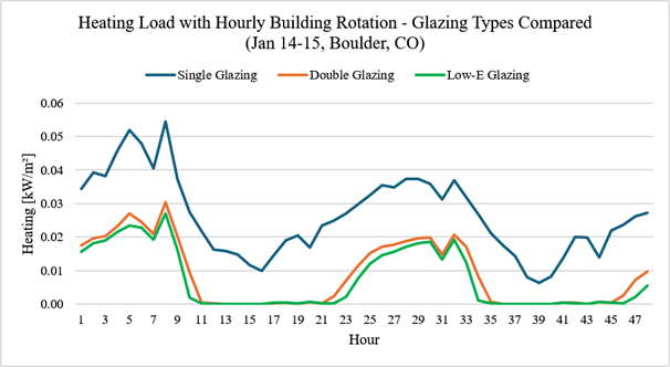
Figure 9 presents hourly heating loads of the housing unit R1 model in Boulder, CO, for two winter days (i.e., January 14–15) for three glazing types. Single glazed housing unit results in the highest heating demand due to the poor thermal performance of the glazed façades. Double and Low-E double glazed facades greatly reduce the heating needs for the housing units. Specifically, Low-E double glazing achieves near-zero heating demand during several hours of the two-day period when solar gains meet all the heating needs for the housing units.

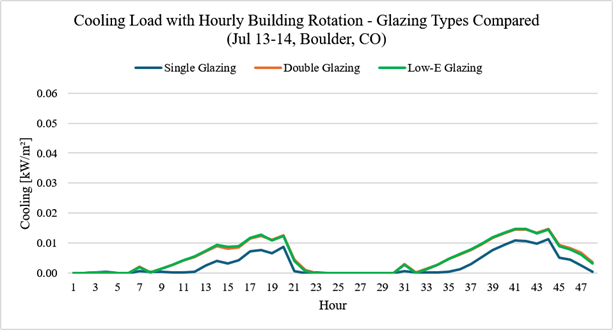
Figure 10 shows the variations of cooling energy demands for hourly rotating housing units R1 model in Boulder, CO, during July 13–14 using three glazing types. Surprisingly, single glazed housing units exhibit the lowest cooling demands despite the high SHGC of the windows. This result is due to the high U-value of the single glazed fenestration system allowing faster night-time heat dissipation, reducing the next day’s heat gain buildup for the housing unit. Higher performing glazing types (i.e., double and Low-E double) traps more heat, leading to higher peak cooling demand for the housing unit, even though they reduce direct solar gains.

Table 9. Effects of WWR on annual heating and cooling energy demands for housing unit R1 Model in Boulder, CO

WWR	Orientation Strategy	Space Heating and Cooling Energy [kWh/\(m^2\)]	Reduction vs Static [%]
0.1	Optimal Static	101.48	–
	Monthly Rotation	100.54	0.9%
	Daily Rotation	100.48	1.0%
	Hourly Rotation	100.23	1.2%
0.2	Optimal Static	94.03	–
	Monthly Rotation	92.15	2.0%
	Daily Rotation	92.00	2.2%
	Hourly Rotation	91.38	2.8%
0.3	Optimal Static	87.46
	Monthly Rotation	84.57	3.3%
	Daily Rotation	84.31	3.6%
	Hourly Rotation	83.29	4.8%
0.4	Optimal Static	81.46	–
	Monthly Rotation	77.40	5.0%
	Daily Rotation	77.05	5.4%
	Hourly Rotation	75.70	7.1%
0.5	Optimal Static	75.94	–
	Monthly Rotation	70.59	7.0%
	Daily Rotation	70.20	7.6%
	Hourly Rotation	68.62	9.6%
0.6	Optimal Static	71.21	–
	Monthly Rotation	64.62	9.2%
	Daily Rotation	64.16	9.9%
	Hourly Rotation	62.47	12.3%
0.7	Optimal Static	67.25	–
	Monthly Rotation	59.43	11.6%
	Daily Rotation	58.91	12.4%
	Hourly Rotation	57.16	15.0%
0.8	Optimal Static	63.88	–
	Monthly Rotation	54.80	14.2%
	Daily Rotation	54.24	15.1%
	Hourly Rotation	52.52	17.8%
0.9	Optimal Static	61.08	–
	Monthly Rotation	50.86	16.7%
	Daily Rotation	50.30	17.6%
	Hourly Rotation	48.58	20.5%

Table 10. Impact of glazing type on annual heating and cooling demands for static and rotating housing unit R1 model in Boulder, CO

ID	Glazing Type	U-Value [W/\(m^2\)·K]	SHGC	Orientation Strategy	Space Heating and Cooling Energy [kWh/\(m^2\)·year]	Reduction vs Static [%]
R1	Single Glazing	5.7	0.85	Optimal Static	139.94	–
				Monthly Rotation	137.19	2.0%
				Daily Rotation	136.75	2.3%
				Hourly Rotation	134.39	4.0%
R1	Double Glazing	1.1	0.65	Optimal Static	63.88	–
				Monthly Rotation	54.80	14.2%
				Daily Rotation	54.24	15.1%
				Hourly Rotation	52.52	17.8%
R1	Low-E Glazing	1.1	0.55	Optimal Static	58.51	–
				Monthly Rotation	48.82	16.6%
				Daily Rotation	48.08	17.8%
				Hourly Rotation	45.82	21.7%

3.5 Impact of Location and Climate

To evaluate the energy effectiveness of building rotation for various locations and climates, a series of analyses are conducted using the housing unit R1 model for several worldwide cities spanning low, mid, and high latitudes. Each city presents distinct solar conditions, heating/cooling demands, and seasonal variabilities. Uniform heating and cooling temperature setpoints were applied across all locations to ensure consistent comparison of rotation effects under different climatic conditions as detailed in Table 11.

Table 11. Heating and cooling setpoints used in all simulations

Parameter	Value
Heating setpoint	21 °C
Cooling setpoint (occupied)	24 °C
Cooling setback (unoccupied)	26.7 °C

Table 12, Table 13, and Table 14 summarize annual energy use and the impact of monthly, daily, and hourly rotation adjustments across various cities grouped into three latitude sets.

For low-latitude regions such as Quito, Ecuador, Bogota, Colombia, Guatemala City, Guatemala, and Caracas, Venezuela, the energy use for the housing unit R1 model is dominated by cooling needs with minimal or no heating demands. Building rotation in these climates helps reduce solar exposure, leading to significant annual energy savings compared to static units (up to 77% in Quito, Ecuador, 58% in Bogota, Colombia, and 53% in Guatemala City, Guatemala). However, because the baseline energy consumption is already low, the absolute annual energy savings remain modest for the housing units (i.e., 3–4 kWh/\(m^2\)·year).

A notable exception is Caracas, Venezuela, where the baseline cooling energy demand is over 100 kWh/\(m^2\). Although rotating the housing unit achieves only a 6% reduction, this still translates into a substantial absolute reduction of 6.78 kWh/\(m^2\). Similarly, the climate of Honolulu, HI, results in high year-round cooling demand for the housing unit R1 model and a significant impact for rotating the unit with a meaningful reduction in annual energy needs of 7.5 kWh/\(m^2\) using hourly orientation adjustments.

For mid-latitude locations, such as Boulder, CO, Albuquerque, NM, and New Orleans, LA, rotating the housing units offer the highest potential for both absolute and relative energy savings compared to their static counterparts. Indeed, these climates require both heating and cooling for the housing units, making them well suited to dynamic orientation strategies.

For a housing unit in Albuquerque, NM, the annual energy needs are reduced by 30% (16 kWh/\(m^2\)) using hourly rotation due mostly to reduced summer cooling demands. Rotating a housing unit in New Orleans, LA, lowers heating needs during the winter period (reduced from 18.14 to 7.16 kWh/\(m^2\)). A rotating housing unit in Boulder, CO, achieves energy savings for both heating and cooling demands as indicated in Table 12.

For cities such as Miami, FL, with cooling dominated climates, rotating residential buildings provide only minor energy benefits with reduction of around 4% in annual energy demands compared to static cases even when hourly orientation adjustments are considered as shown in Table 13.

Table 12. Energy performance of rotating buildings compared to their static counterparts in tropical and equatorial climates (i.e. locations with latitude ranging from 0° to 20°)

Location	Orientation Strategy	Space Heating and Cooling Energy [kWh/\(m^2\)]	Heating Load [kWh/\(m^2\)]	Cooling Load [kWh/\(m^2\)]	Reduction vs Static [%]
Quito, Ecuador	Optimal Static (247.5°)	4.78	2.02	2.76	–
(Latitude 0°)	Monthly Rotation	3.68	2.16	1.52	23%
	Daily Rotation	2.11	1.34	0.77	56%
	Hourly Rotation	1.08	0.93	0.15	77%
Bogota, Colombia	Optimal Static (270°)	5.50	3.09	2.41	–
(Latitude 5°)	Monthly Rotation	5.08	3.49	1.59	8%
	Daily Rotation	3.67	2.71	0.96	33%
	Hourly Rotation	2.29	2.07	0.22	58%
Caracas, Venezuela	Optimal Static (0.0°)	105.27	0.00	105.27	–
(Latitude 10°)	Monthly Rotation	98.68	0.00	98.68	6%
	Daily Rotation	98.49	0.00	98.49	6%
	Hourly Rotation	98.49	0.00	98.49	6%
Guatemala City, Guatemala	Optimal Static (0.0°)	6.05	0.60	5.45	–
(Latitude 15°)	Monthly Rotation	3.37	0.43	2.94	44%
	Daily Rotation	3.00	0.12	2.88	50%
	Hourly Rotation	2.85	0.04	2.81	53%
Honolulu, HI	Optimal Static (0.0°)	45.56	0.03	45.53	–
(Latitude 20°)	Monthly Rotation	42.06	0.03	42.03	8%
	Daily Rotation	41.84	0.03	41.81	8%
	Hourly Rotation	38.10	0.01	38.09	16%

Table 13. Energy performance of rotating buildings compared to their static counterparts in temperate and semi-arid climates (i.e. locations with latitude ranging from 25° to 40°)

Location	Orientation Strategy	Space Heating and Cooling Energy [kWh/\(m^2\)]	Heating Load [kWh/\(m^2\)]	Cooling Load [kWh/\(m^2\)]	Reduction vs Static [%]
Miami, FL	Optimal Static (0.0°)	58.45	0.86	57.59	–
(Latitude 25°)	Monthly Rotation	56.89	0.86	56.03	3%
	Daily Rotation	56.33	0.34	55.99	4%
	Hourly Rotation	56.08	0.26	55.82	4%
New Orleans, LA	Optimal Static (0.0°)	55.53	18.14	37.39	–
(Latitude 30°)	Monthly Rotation	48.79	9.30	39.49	12%
	Daily Rotation	45.75	7.88	37.87	18%
	Hourly Rotation	44.40	7.16	37.24	20%
Albuquerque, NM	Optimal Static (180°)	52.76	25.49	27.27	–
(Latitude 35°)	Monthly Rotation	43.07	26.45	16.62	18%
	Daily Rotation	40.24	25.65	14.59	24%
	Hourly Rotation	36.77	23.74	13.03	30%
Boulder, CO	Optimal Static (180°)	63.88	49.89	13.99	–
(Latitude 40°)	Monthly Rotation	54.80	48.47	6.33	14%
	Daily Rotation	54.24	47.91	6.33	15%
	Hourly Rotation	52.52	46.38	6.14	18%

Table 14. Energy performance of rotating buildings compared to their static counterparts in colder and oceanic climates (i.e. locations with latitude higher than 40o)

Location	Orientation Strategy	Space Heating and Cooling Energy [kWh/\(m^2\)]	Heating Load [kWh/\(m^2\)]	Cooling Load [kWh/\(m^2\)]	Reduction vs Static [%]
Minneapolis, MN	Optimal Static (180°)	194.52	178.75	15.77	–
(Latitude 45°)	Monthly Rotation	186.45	178.33	8.12	4%
	Daily Rotation	185.54	177.47	8.07	5%
	Hourly Rotation	183.00	175.14	7.86	6%
Bellingham, WA	Optimal Static (180°)	67.38	63.07	4.31	–
(Latitude 50°)	Monthly Rotation	64.08	63.17	0.91	5%
	Daily Rotation	62.70	62.05	0.65	7%
	Hourly Rotation	61.29	60.91	0.38	9%
Glasgow, United Kingdom	Optimal Static (180°)	74.15	73.62	0.53	–
(Latitude 55°)	Monthly Rotation	73.38	72.71	0.67	1%
	Daily Rotation	72.36	72.04	0.32	2%
	Hourly Rotation	71.06	70.94	0.12	4%

For high-latitude cities such as Minneapolis, MN, Bellingham, WA, and Glasgow, United Kingdom, annual energy demands for the housing units are primarily driven by heating needs. While rotation yields measurable annual energy reductions (up to 9% for buildings in Bellingham, WA), its overall impact remains limited as depicted by the results summarized in Table 14. This is largely due to the low winter sun angles and already optimal orientations (typically south) used for static buildings, which constrain the added value of any rotation strategy.

4. Integrated Rotating Buildings with Photovoltaic Systems

This section explores the combined impacts of building rotation and photovoltaic (PV) tracking strategies on the overall energy performance of residential buildings. Specifically, rooftop PV systems are integrated with rotating residential buildings described in Section 2. The rooftop PV panels can be either fixed or dynamic using azimuth and/or tilt tracking systems.

Three configurations of integrated PV rotating residential buildings are considered in the assessment analysis: (A) a static building with dual‑axis PV tracking system; (B) a rotating building with fixed rooftop PV system; and (C) a rotating building and independent tracking PV system. Initially, the analysis of the three configurations of the integrated PV rotating residential buildings was carried out for Boulder, CO, and the R2 building geometry. Then, a broader cross‑climate comparative assessment for the three configurations of the integrated PV rotating buildings is performed using the R1 building geometry to develop some basic guidelines on the best climatic conditions suitable for rotating buildings.

4.1 Comparative Analysis for Integrated PV Rotating Buildings

This section evaluates the energy performance of three integrated PV building configurations in Boulder, CO, using the R2 building geometry, comprising of one static configuration and two rotating configurations. The net energy balance is expressed both in absolute terms (kWh/year) and as a percentage of the annual energy demand of rotating building relative the corresponding static configuration. Positive values indicate an annual energy surplus, whereas negative values indicate an annual energy deficit.

4.1.1 Scenario A: Static Building with Dual-Axis PV Tracking System

This scenario evaluates a static residential building equipped with a dual‑axis rooftop PV system that continuously tracks the sun to maximize annual electricity generation. The static building is set at its optimal orientation (i.e., south), while the PV panels adjust both azimuth and tilt throughout the year.

Two roof coverage levels are evaluated in this analysis as outlined in Table 15. The first option uses 25 modules (i.e., 8.18 kW) resulting in 40 % roof coverage, achieving near net‑zero operation. While the second option increases PV roof coverage to 48 % using 30 modules (i.e., 9.81 kW), generating a significant annual energy surplus for the building as summarized in Table 15.

Table 15. Net annual energy balance for Scenario A (static building with dual-axis PV tracking), Boulder, CO

PV Roof Coverage [%]	Building Rotation Strategy	Net Energy Balance [kWh/\(m^2\)·year]	Net Energy Balance [% Of Annual Building Demand]
40%	Static	0.35	0.4
48%	Static	16.51	20.5

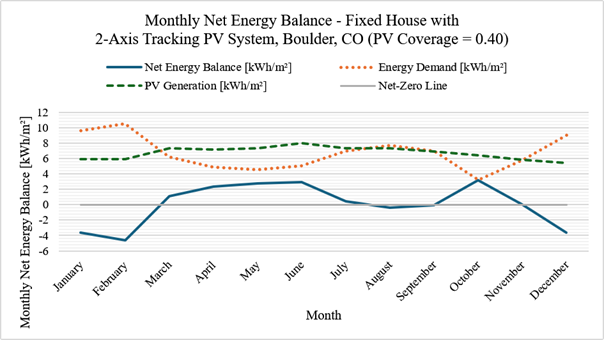
Figure 11 and Figure 12 illustrate the monthly building energy demand, PV electricity generation, and resulting net energy balance for the integrated static PV building in Boulder, CO, for roof coverage of 40% and 48%, respectively. As shown in Figure 11, when the PV coverage is 40%, the static residential building achieves net‑zero energy performance annually but exhibits strong seasonal energy imbalances. Specifically, the building during the winter months (January–February) shows energy deficits. While during the summer months, the building generates significant electricity surpluses, yielding annually about 0.35 kWh/\(m^2\)·year in net energy gains.

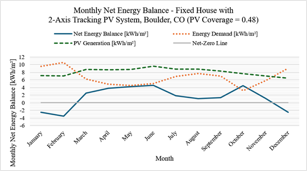
When the PV roof coverage is 48%, higher electricity generation is achieved on monthly basis as noted in Figure 12 resulting in an annual surplus of 16.51 kWh/\(m^2\)·year for the static building.

4.1.2 Scenario B: Rotating Building with Fixed Rooftop PV

This scenario evaluates the performance of a rotating residential building with rooftop PV panels mounted at a fixed 35° tilt. Thus, the rooftop PV array has a constant tilt and azimuth relative to the roof, but its solar exposure varies with the rotating building’s orientation. Two PV roof coverage levels are considered 40% (i.e., PV capacity of 8.175 kW) and 48% (i.e., PV capacity of 9.81 kW). Table 16 summarizes the annual energy balance for the integrated PV rotating building under three rotation adjustment frequencies (monthly, daily, and hourly) and two PV roof coverage levels (40% and 48%).

Table 16. Net annual energy balance for Scenario B (rotating building with fixed rooftop PV system), Boulder, CO

PV Roof Coverage [%]	Building Rotation Strategy	Net Energy Balance [kWh/\(m^2\)·year]	Net Energy Balance [% Of Annual Building Demand]
40%	Monthly	0.83	1.2
	Daily	2.18	3.0
	Hourly	9.48	13.2
48%	Monthly	15.32	21.4
	Daily	17.04	23.5
	Hourly	25.78	35.7

Compared to Scenario A, rotating the building significantly improves its energy performance, especially using hourly orientation adjustments even with fixed rooftop PV system. For PV roof coverage of 40%, the net annual energy balance for the rotating building with fixed rooftop PV reaches up to 9.48 kWh/\(m^2\)·year, significantly higher than the 0.35 kWh/\(m^2\)·year achieved for Scenario A. When the PV roof coverage is 48%, the rotating building integrated with fixed rooftop PV panels has a net energy surplus of 25.78 kWh/\(m^2\)·year due to higher electricity generated by the PV array.

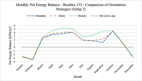
Figure 13 shows the monthly net energy balance for the integrated PV rotating building when the PV roof coverage is 48% for three rotating adjustment frequencies. From March to October, the hourly rotation achieved significantly higher net energy yield than monthly or daily rotation setting strategies. This higher energy performance is due to the benefits of solar tracking which enhances both PV output generation and building energy efficiency.

During January and February, all rotation strategies performed similarly, as the optimal building orientation during this winter period remains south-facing to maximize solar gains and reduce heating needs. During warmer months, hourly adjustments of the orientation of the building enable to capture morning/evening solar heat gains while reducing afternoon overheating by turning the façade away from peak sun angles as well as maintaining high yields for the rooftop PV system.

4.1.3 Scenario C: Independently Rotating Building and Rooftop PV System

This scenario combines dynamic building rotation with dual-axis tracking rooftop PV system, allowing both systems to optimize their respective energy performance independently. While the tracking PV array continuously follows the sun through adjustments of both its tilt and azimuth, the building is rotated monthly, daily, or hourly to minimize its heating and cooling thermal loads.

Table 17 summarizes the annual energy balance for the integrated PV rotating building under different rotation strategies and PV roof coverage levels.

All integrated PV rotating building configurations achieve significant energy surpluses. For PV roof coverage of 40%, hourly rotation settings yield an annual net energy surplus of 10.57 kWh/\(m^2\)·year. For PV roof coverage of 48%, the annual net energy surplus is 25.87 kWh/\(m^2\)·year due to higher electricity generation. However, the differences in energy performance between monthly, daily, and hourly rotation frequency strategies are modest since all the cases benefit from the high electricity yields achieved by the tracking PV system. Figure 14 illustrates the monthly building energy demand, PV electricity generation, and resulting net energy balance for the integrated PV rotating building in Boulder, CO, under hourly orientation settings and 48% PV roof coverage. Positive net energy balances are achieved for most of the months with only December, January, and February having small energy deficits due to low solar irradiance and higher heating demands.

Table 17. Net annual energy balance for Scenario C, (rotating building with independently tracking rooftop PV system), Boulder, CO

PV Roof Coverage [%]	Building Rotation Strategy	Net Energy Balance [kWh/\(m^2\)·year]	Net Energy Balance [% Of Annual Building Demand]
40%	Monthly	9.71	13.7
	Daily	9.97	14.1
	Hourly	10.57	14.9
48%	Monthly	25.87	36.4
	Daily	26.13	36.9
	Hourly	26.73	37.9

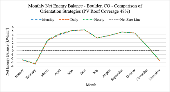
In summary, Scenario C provides the highest energy performance among the evaluated configurations, although the magnitude of the benefits varies depending on climate and building characteristics. Since the PV tracking system maximizes electricity yield, most of the added value of rotating the building can be achieved using only monthly orientation adjustments.

4.1.4 Comparative Analysis

Table 18 summarizes the annual net energy balance for all three scenarios of dynamic PV-integrated buildings in Boulder, CO, considering two PV rooftop capacities (40% PV roof coverage with 8.18 kW and 48% PV roof coverage with 9.81 kW) and the three building rotation adjustment frequencies (monthly, daily, and hourly).

As indicated in Table 18 the configurations involving building rotation (Scenarios B and C) outperformed the static building configurations (Scenario A), particularly using hourly orientation settings. For instance, when the PV roof coverage is 40%, the annual energy surplus increases from only 0.35 kWh/\(m^2\)·year for Scenario A to 9.48 kWh/\(m^2\)·year for Scenario B, and 10.57 kWh/\(m^2\)·year for Scenario C using hourly orientation adjustments.

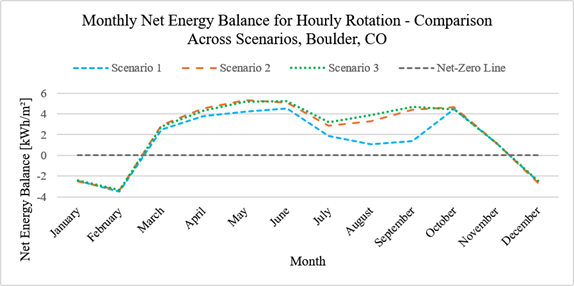
Figure 15 shows the monthly variations of the net energy balance for three PV-integrated building configurations in Boulder, CO, using dual tracking PV system and hourly orientation settings for rotating building cases. These results demonstrate that incorporating rotation strategies substantially enhances the overall energy performance of residential buildings compared to traditional static structures, even when PV tracking system is used. The differences in annual energy performance between Scenarios B and C building configurations are moderate since both benefits from building rotating and PV tracking. However, the same differences between Scenarios B or C and Scenario A are more significant, indicating that dynamic building rotation offers substantial energy benefits especially using hourly orientation settings.

As noted in Figure 15, Scenarios B and C clearly outperform Scenario A during March through September with lower net energy balance for the PV-integrated building in Boulder, CO. This improvement stems from the combined benefits of optimized PV yields and reduced building thermal loads through dynamic orientation adjustments. During winter months, there is no benefit of rotating the building in Boulder, CO, as the south orientation consistently provides the lowest heating thermal loads compared to other orientations.

Table 18. Summary of annual net energy balances for all PV-integrated building configuration , Boulder, CO

Scenario	PV Roof Coverage	Building Rotation Strategy	Building Energy Needs [kWh/\(m^2\)·year]	PV Outputs [kWh/\(m^2\)·year]	Net Energy Balance [kWh/\(m^2\)·year]		Net Energy Balance [% Of Annual Building Demand]
A	40%	Static	80.46	80.81		0.35	0.4
A	48%	Static	80.46	96.97		16.51	20.5
B	40%	Monthly	71.63	71.45		0.83	1.2
		Daily	71.79	73.97		2.18	3.0
		Hourly	71.93	81.41		9.48	13.2
B	48%	Monthly	71.63	86.94		15.32	21.4
		Daily	71.79	88.76		17.04	23.5
		Hourly	71.93	97.69		25.78	35.7
C	40%	Monthly	71.10	80.81		9.71	13.7
		Daily	70.84	80.81		9.97	14.1
		Hourly	70.31	80.81		10.57	14.9
C	48%	Monthly	71.10	96.97		25.87	36.4
		Daily	70.84	96.97		26.13	36.9
		Hourly	70.31	96.97		26.73	37.9

While Scenarios B and C demonstrate improved energy performance compared to Scenario A, these benefits should also be evaluated based on practical trade-offs and multiple performance criteria. Rotating buildings and PV tracking systems introduce additional mechanical complexity, which may result in higher initial construction costs, increased maintenance requirements, and potential reliability concerns. Frequent rotation strategies (i.e., hourly adjustments) may lead to increased deterioration and operational constraints for the rotating systems. From an occupant perspective, continuous or frequent building rotation could also raise concerns related to comfort, perception of movement, and usability of interior spaces. Therefore, while Scenario C provides the highest energy performance, its practical implementation may require careful consideration using multiple criteria including energy efficiency, economic feasibility, system durability, and user acceptance. In some cases, simpler configurations such as Scenario A or limited rotation strategies may offer a more balanced compromise between energy performance and practical feasibility.

4.2 Climate Impacts

This section examines the annual energy performance of dynamic PV-integrated buildings for a range of climates across different regions of the world. The analysis considers the R1 residential building model with a 100 \(m^2\) floor area and a rectangular shape. The PV roof coverage is set 30% (i.e., PV capacity of 5.89 kW) for all building configurations A, B, and C as described in Section 4. Moreover, the analysis is carried out for 13 cities located in various regions in the world with varying latitudes and climates.

The analysis results are summarized in Table 19 providing the annual net energy demands for PV-integrated static (Scenario A) and rotating (Scenarios B, and C) buildings achieved for all 13 cities using three building rotation frequencies. The color scale highlights ratings of the annual energy performance levels for each location. Green represents the best energy performing case while red indicates the case with the lowest energy benefits.

Table 19. Annual net energy Balances [kWh/\(m^2\)·year] for PV-integrated static and rotating buildings located in 13 cities for three scenarios and three orientation adjustment frequencies

City (Latitude)	Scenario A [kWh/ m\(^2\!\cdot\)year]	Scenario B Monthly [kWh/ m\(^2\!\cdot\)year]	Scenario B Daily [kWh/ m\(^2\!\cdot\)year]	Scenario B Hourly [kWh/ m\(^2\!\cdot\)year]	Scenario C Monthly [kWh/ m\(^2\!\cdot\)year]	Scenario C Daily [kWh/ m\(^2\!\cdot\)year]	Scenario C Hourly [kWh/ m\(^2\!\cdot\)year]
Quito, Ecuador (0\(^\circ\))	55.73	56.76	58.51	64.48	60.26	61.80	62.04
Bogota, Colombia (5\(^\circ\))	51.87	49.29	50.51	56.66	52.27	53.65	54.32
Caracas, Venezuela (10\(^\circ\))	-34.26	-42.23	-41.45	-32.61	-27.69	-27.54	-28.23
Guatemala City, Guatemala (15\(^\circ\))	78.67	64.89	68.29	80.89	81.34	81.67	81.03
Honolulu, HI (20\(^\circ\))	39.92	13.89	18.38	37.51	43.42	43.68	46.64
Miami, FL (25\(^\circ\))	17.93	-8.15	-1.95	14.08	19.47	19.99	19.54
New Orleans, LA (30\(^\circ\))	22.59	11.43	15.00	25.29	29.33	32.33	32.98
Albuquerque, NM (35\(^\circ\))	46.80	43.82	45.07	60.14	56.49	59.27	61.96
Boulder, CO (40\(^\circ\))	11.80	8.91	10.82	21.95	20.86	21.38	22.39
Minneapolis, MN (45\(^\circ\))	-133.96	-138.27	-136.00	-125.13	-125.90	-125.03	-123.28
Bellingham, WA (50\(^\circ\))	-22.59	-26.96	-24.69	-16.47	-19.30	-17.96	-17.27
Glasgow, United Kingdom (55\(^\circ\))	-56.92	-60.18	-58.48	-53.65	-56.16	-55.18	-54.60

For equatorial and low-latitude cities (e.g., Quito, Ecuador, Bogota, Colombia, Guatemala City, Guatemala), all building configurations using Scenario A perform well due to high and consistent availability of solar irradiance throughout the year resulting in significant PV electricity yields. The addition of building rotation in these cities (i.e., building configurations using Scenarios B and C) achieve limited energy benefits. For Bogota, Colombia and Guatemala City, Guatemala, monthly and daily rotation (Scenario B) strategies have even decreased slightly the energy benefits of the rotating buildings compared to their static cases. Hourly rotation strategies (Scenario B-hourly or Scenario C-hourly) yielded modest energy improvements, typically under 5.00 kWh/\(m^2\)·year, which may not justify the added mechanical complexity of rotating buildings in these climates. Notable exceptions include Quito, Ecuador, where Scenario B-hourly outperformed Scenario A by nearly 9.00 kWh/\(m^2\)·year, benefiting from seasonal variations of solar gains and heating demands. Dynamic PV-integrated buildings in Caracas, Venezuela, located near the equator, exhibit limited energy benefits compared to static buildings due to the consistently high cooling loads through the year. Only buildings using Scenario C and rotated using hourly orientation settings achieve a positive net energy surplus of about 6.00 kWh/\(m^2\)·year compared to the static buildings

For tropical locations (i.e., Miami, FL, Honolulu, HI), similar energy performance patterns are achieved by all the PV-integrated building configurations. Buildings using Scenario A consistently outperform those using Scenario B, even when using hourly rotation adjustment frequency. For instance, Miami, FL, dynamic buildings using Scenario B located in Miami, FL, with monthly and daily rotation options result in significantly higher annual net energy demands estimated at -8.15 kWh/\(m^2\)·year and -1.95 kWh/\(m^2\)·year, respectively. However, when hourly rotation settings are deployed, buildings using Scenario B achieve annual energy surplus in Miami, FL. Buildings using Scenario C have the best energy performance in Miami, FL, especially when hourly rotation frequency is used.

In contrast, for mid-latitude cities (e.g., Albuquerque, NM, Boulder, CO, New Orleans, LA), rotating buildings exhibit substantial energy benefits compared to static options. For instance, buildings using Scenario B and Scenario C in Albuquerque, NM, achieve annual net energy surpluses of over 13.00 kWh/\(m^2\)·year and 15.00 kWh/\(m^2\)·year, respectively, compared to buildings using Scenario A. Similarly, PV-integrated rotating buildings in Boulder, CO, result in substantial energy benefits with more than 22.00 kWh/\(m^2\)·year in annual net energy surplus. These climates, characterized by mixed heating and cooling thermal needs for the buildings and moderate solar availability, are favorable for orientation-adaptive strategies.

For cities located at higher latitudes (i.e., Minneapolis, MN, Bellingham, WA, Glasgow, United Kingdom), characterized by limited solar availability and long heating seasons, only limited energy benefits are obtained from dynamic PV-integrated buildings with 30% PV roof coverage. Nevertheless, rotating buildings with tracking PV systems can reduce substantially the annual energy demands compared to the static building configurations, especially when hourly orientation settings are deployed. For instance, building configurations using Scenario B and Scenario C in Minneapolis, MN, have annual net energy demands reduced by over 10.00 kWh/\(m^2\)·year compared to those using Scenario A. Similar results are found for PV-integrated rotating buildings in Bellingham, WA and Glasgow, United Kingdom even their energy benefits are lower.

Overall, the analysis results summarized in Table 19 indicate that building rotation strategies are most effective when applied using hourly orientation settings and located in climates with seasonal variability and mixed thermal demands. Building configurations using Scenario C consistently provided the highest net energy benefits compared to those using Scenario B and especially Scenario A.

5. Summary and Conclusions

This study evaluated the energy performance of rotating residential buildings through an integrated analysis framework that combines building thermal load estimations, photovoltaic (PV) electricity yield calculations, and dynamic building orientation optimizations. By analyzing building rotation effects both separately and in combination with PV tracking systems, the framework aims to determine whether rotating buildings can provide meaningful energy benefits across a wide range of global climates. The results demonstrate that building rotation, when combined with dual-axis PV tracking systems, can significantly improve the net energy performance of residential buildings, particularly in climates with balanced heating and cooling demands.

The evaluation of rotating buildings without PV showed that orientation has a substantial impact on thermal loads, especially in mid-latitude climates where seasonal differences in solar altitude are pronounced. Across the building geometries analyzed, elongated shapes exhibited the strongest response to dynamic rotation due to their large directional differences in façade exposures. For Boulder, CO, the two-story rectangular buildings can achieve up to 24% annual energy savings using hourly optimized orientation settings compared to their optimal static orientation. Buildings with high glazed areas further amplify the energy benefits of dynamic orientation settings due to the increased influence of solar heat gains on both heating and cooling loads. In contrast, compact or radially symmetric geometries such as squares or octagons showed limited sensitivity to dynamic building rotation even when hourly orientation settings are considered with annual energy reductions of less than 6%. Moreover, the analysis indicates that glazing type plays a significant role in the energy benefits of rotating buildings. Rotating buildings with low-emissivity double glazing outperformed those with single and standard double glazing by reducing winter heat losses and improving the benefits of passive solar gains compared to static buildings especially those oriented south-east and south-west.

When integrating rotating buildings with dynamic rooftop PV systems, the analysis indicates that their energy benefits depend strongly on the climate. Three building configurations were evaluated: (i) Scenario A for static buildings equipped with dual-axis PV tracking systems, (ii) Scenario B for rotating buildings with fixed rooftop PV arrays, and (iii) Scenario C coupling rotating buildings with independently tracking dual-axis PV systems. Across all climates considered, Scenario C generally provides the highest annual net energy performance among the evaluated configurations, although the magnitude of the benefits varies depending on climate. In mid-latitude regions, buildings using Scenario C can achieve large annual energy surpluses, exceeding 25 kWh/\(m^2\)·year when located in Boulder, CO, for a 9.81 kW rooftop PV system. For low-latitude locations, the energy benefits of rotating buildings are limited, as solar availability remains relatively constant throughout the year. In these climates, static buildings using Scenario A can perform similarly to, or even better than, rotating configurations. By contrast, high-latitude locations with significant heating demands can benefit from rotating buildings primarily through seasonal south-facing orientation adjustments.

Overall, the analysis results indicate that rotating buildings can provide substantial energy benefits in regions with balanced heating and cooling thermal demands and high seasonal solar variations. However, the energy benefits of rotating buildings are not uniform across all climates and depend strongly on climatic conditions, building geometry, and operational strategies. For favorable climates, building rotation can provide significant thermal benefits as well as enhance PV electricity generation for fixed rooftop PV systems, especially when hourly building orientation adjustments are considered.

While rotating buildings and PV tracking systems offer significant energy performance benefits, their practical implementation involves several challenges. These systems introduce additional mechanical complexity, which may result in higher initial capital costs, increased maintenance requirements, and potential reliability and durability concerns. For instance, structural considerations, including the design of rotating platforms and load-bearing systems, are critical to ensure safe and durable operation. From an occupant perspective, frequent or continuous rotation may affect comfort, perception of movement, and usability of interior spaces. Therefore, although advanced kinematic building configurations such as those with hourly rotations provide the highest energy performance, their overall effectiveness must be carefully evaluated, and simpler strategies may offer a more practical compromise between energy performance and implementation.

In addition, it is important to recognize that alternative adaptive design strategies may offer similar or even better energy performance improvements with lower mechanical complexity. Solutions such as dynamic shading systems, adaptive façades, or advanced glazing technologies can effectively regulate solar gains and daylight availability while requiring significantly less mechanical infrastructure than full building rotation. These approaches may therefore represent more practical or cost-effective options in certain contexts. Rotating buildings should be considered as one of several possible strategies within the broader framework of adaptive and responsive building design alternatives, rather than as universally optimal solutions.

Future research could expand the scope of the analysis framework to account for a wider range of envelope characteristics, including buildings with high thermal mass. Moreover, the analysis could be extended to evaluate the economic implications of dynamic buildings and PV systems and include especially the costs for the rotating platforms. Indeed, the widespread adoption of rotating residential buildings will depend primarily on developing solutions that are not only energy-efficient but also cost-effective and acceptable to occupants. Nevertheless, this study provides a foundational assessment of the energy benefits of dynamically oriented buildings, especially when coupled with rooftop PV systems, to substantially enhance their energy performance across a wide range of climates worldwide.

Nomenclature

ACH:	Air Change per Hour
COF:	Coefficient Of Performance
DBEM:	Distinct Building Energy Modeling
DHW:	Domestic Hot Water
HSPF:	Heating Seasonal Performance Factor
HVAC:	Heating, Ventilating, and Air Conditioning
PV:	Photovoltaic
SHGC:	Solar Heat Gain Coefficient
WWR:	Window-to-Wall Ratio